Sequence tagging with HMMs, MEMMs and CRFs
I drew inspiration for this blog from Prof. Collin’s excellent write-ups.
Let us consider sequence tagging problems such as POS or NER tagging. Given a sequence of tokens, we would like to predict the most likely (non-observable, hidden) tags that correspond to these tokens.
Let us look at a POS-tagged example:
import nltk

tagged_sentences = nltk.corpus.treebank.tagged_sents()
print(tagged_sentences[0])
print()
print('Number of tagged sentences: %d' % len(tagged_sentences))
print('Number of tagged tokens: %d' % sum([len(tagged_sentence) for tagged_sentence in tagged_sentences]))
print()
unique_tags = set([
    tag
    for tagged_sentence in tagged_sentences
    for _,tag in tagged_sentence])
print('Set of unique tags: %s' % str(unique_tags))
Output:
[('Pierre', 'NNP'), ('Vinken', 'NNP'), (',', ','), ('61', 'CD'), ('years', 'NNS'), ('old', 'JJ'), (',', ','), ('will', 'MD'), ('join', 'VB'), ('the', 'DT'), ('board', 'NN'), ('as', 'IN'), ('a', 'DT'), ('nonexecutive', 'JJ'), ('director', 'NN'), ('Nov.', 'NNP'), ('29', 'CD'), ('.', '.')]

Number of tagged sentences: 3914
Number of tagged tokens: 100676

Set of unique tags: {'.', 'POS', 'NNS', "''", 'JJR', 'LS', 'IN', 'JJ', 'NNP', '``', 'FW', '#', '$', 'WDT', 'WP$', 'PRP', 'VBZ', ',', 'TO', 'VBD', 'SYM', 'JJS', 'VBG', 'RBR', 'PRP$', 'CD', 'MD', '-NONE-', '-LRB-', '-RRB-', 'CC', 'DT', 'NNPS', 'VBN', 'UH', 'RB', 'NN', 'VBP', 'WRB', 'RBS', 'PDT', 'RP', 'WP', ':', 'EX', 'VB'}
During test time, we may be given a token sequence such as ['The', 'cool', 'cat', '.'] and we may be required to predict the most likely tag sequence ['DT', 'JJ', 'NN', '.'].
Hidden Markov Models (HMM)
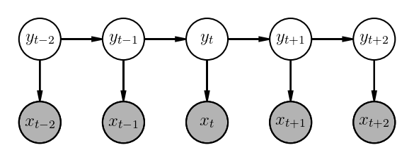
A generative bigram HMM model factors the probability distribution for a given observed token sequence $\underline{x_{1:T}}$ and (hidden, non-observable) tag sequence $\underline{y_{1:T}}$ as follows:
\[p(\underline{x_{1:T}} , \underline{y_{1:T}}) = \prod_{t=1}^{T+1}p(y_t|y_{t-1})\cdot\prod_{t=1}^Tp(x_t|y_t)\]Here is how its graphical model looks like:
 |
|---|
| Space |
A generative trigram HMM model factors the probability distribution for a given observed token sequence $\underline{x_{1:T}}$ and (hidden, non-observable) tag sequence $\underline{y_{1:T}}$ as follows:
\[p(\underline{x_{1:T}} , \underline{y_{1:T}}) = \prod_{t=1}^{T+1}p(y_t|y_{t-1},y_{t-2})\cdot\prod_{t=1}^Tp(x_t|y_t)\]For the above example,
$\underline{x_{1:T}} = $ ['Pierre', 'Vinken', ',', '61', 'years', 'old', ',', 'will', 'join', 'the', 'board', 'as', 'a', 'nonexecutive', 'director', 'Nov.', '29', '.'],
$\underline{y_{1:T}} = $ ['NNP', 'NNP', ',', 'CD', 'NNS', 'JJ', ',', 'MD', 'VB', 'DT', 'NN', 'IN', 'DT', 'JJ', 'NN', 'NNP', 'CD', '.'].
Please note that $y_0 = y_{-1} =$ <START>, a special start tag and $y_{T+1} = $ <EOS>, a special end of sentence (EOS) tag.
- $p(y_t|y_{t-1},y_{t-2})$ denotes the probability of transitioning to tag $y_t$ from preceeding tags $(y_{t-1}, y_{t-2})$. For e.g., you would expect $p(\text{NN}|\text{JJ},\text{DT})$ to be larger as
DT JJ NNdenotes a common noun phraseNPoccurance such asThe (DT) cool (JJ) cat (NN). - $p(x_t|y_t)$ denotes the probability of observing token $x_t$ given the tag is $y_t$. For e.g. you would expect $p(\text{The}|\text{DT})$ to be high, but $p(\text{The}|\text{VB})$ to be low.
How do you estimate these probabilities? Since, if we had these, we could (hypothetically) enumerate over all possible tag sequences $\underline{y_{1:T}}$ and select the one that yeilds the highest probability of the joint distribution.
\[\widehat{\underline{y_{1:T}}} = \underset{\underline{y_{1:T}}}{\operatorname{argmax}} p(\underline{x_{1:T}} , \underline{y_{1:T}})\]with $\widehat{y_0}$, $\widehat{y_{-1}}$ and $\widehat{y_{T+1}}$ fixed to their resp. values as described above. This process of figuring out the most likely tag sequence is called as decoding.
Estimating count based maximum likelihood probabilities is straightforward. For e.g. $p_{ML}(\text{NN}|\text{JJ},\text{DT})$ can be computed from trigram and bigram counts $count(\text{DT}, \text{JJ}, \text{NN})$ and $count(\text{DT}, \text{JJ})$.
\[p_{ML}(\text{NN}|\text{JJ},\text{DT}) = \frac{count(\text{DT}, \text{JJ}, \text{NN})}{count(\text{DT}, \text{JJ})}\]Various smoothing techniques can be used for better generalization.
For e.g.,
\[p_{smoothed}(\text{NN}|\text{JJ},\text{DT}) = \lambda_1\cdot p_{ML}(\text{NN}|\text{JJ},\text{DT}) + \lambda_2\cdot p_{ML}(\text{NN}|\text{JJ}) + \lambda_3\cdot p_{ML}(\text{NN})\]This can deal with missing trigram combinations as well as make use of bigram combinations. The $\lambda$ parameters can be learnt.
How do we deal with out of vocabulory terms while decoding? We assigne them to a special <UNK> token. While training, all the tokens with occurence counts below a certain threshold are converted to <UNK> token. We can further do preprocessing such as convert all 4-digit year occurences (such as 1985 or 2019) to a special <NUM-4> token so that we are able to process previously unforeseen 4-digit year occurence while testing on a new data point.
While this formulation is cool, it ignores a lot of lexical and morphological evidence present in the tokens (and tags). For e.g., a token ending with -er is most likely a comparative adjective (JJR) such as bigger and one ending with -est, a superlative adjective JJS such as biggest. How do we incorporate this sort of information?
We could change the formuation of HMMs as follows. The transition probabilities are obtained as follows:
\[score(y_{t-2},y_{t-1}, y_t, t) = \sum_{k=1}^{K} w_k \cdot f_k(y_{t-2},y_{t-1}, y_t, t) \\ p(y_t|y_{t-1},y_{t-2},\underline{\theta}) = \frac{e^{score(y_{t-2},y_{t-1}, y_t, t)}}{\sum_{\widetilde{y}} e^{score(y_{t-2},y_{t-1}, \widetilde{y}, t)}}\]Similarly, the emission probabilities are obtained as follows:
\[score(x_t, y_t, t) = \sum_{d=1}^{D} v_d \cdot g_d(x_t,y_t, t) \\ p(x_t|y_t,\underline{\theta}) = \frac{e^{score(x_t, y_t, t)}}{\sum_{\widetilde{y}} e^{score(x_t, \widetilde{y}, t)}}\]where $\underline{\theta} = [{\underline{w_{1:K}}; \underline{v_{1:D}}}]$ are the parameters of the model.
The features $f_k(y_t,y_{t-1},y_{t-2}, t)$ and $g_d(x_t, y_t, t)$ are designed to capture prominent morphological and lexical and unigram, bigram, trigram token and tag occurence variations. As an example, consider following features:
\[\begin{equation} f_{112}(y_{t-2}, y_{t-1}, y_t, t)=\left\{ \begin{array}{@{}ll@{}} 1, & \text{if}\ y_t \in [\text{NN, NNS}], y_{t-2}=\text{DT}, y_{t-1} \in [\text{JJ, JJR, JJS}] \\ 0, & \text{otherwise} \end{array}\right. \end{equation}\]This captures the tag sequence for a variation of noun phrase (NP) such as The cool cat.
This captures the tag sequence for a sentence beginning with a noun.
\[\begin{equation} f_{5}(y_{t-2}, y_{t-1}, y_t, t)=\left\{ \begin{array}{@{}ll@{}} 1, & \text{if}\ y_t=\text{VBG}, y_{t-1}=\text{VGZ}, y_{t-2}=\text{NN} \\ 0, & \text{otherwise} \end{array}\right. \end{equation}\]This captures tag trigram occurrence (Idea (NN) is (VGZ) working (VBG)`).
Similarly, consider:
\[\begin{equation} g_{35}(x_t, y_t, t)=\left\{ \begin{array}{@{}ll@{}} 1, & \text{if}\ y_t \in [\text{JJR, JJS}], x_t[-2:] \in [\text{er, es}] \\ 0, & \text{otherwise} \end{array}\right. \end{equation}\] \[\begin{equation} g_{4}(x_t, y_t, t)=\left\{ \begin{array}{@{}ll@{}} 1, & \text{if}\ y_t=\text{NNS}, x_t[-1]=\text{s} \\ 0, & \text{otherwise} \end{array}\right. \end{equation}\]$g_{35}$ captures the occurence of comparative or superlative adjectives where as $g_{4}$ captures the plural form of nouns.
The parameters of this model are $\underline{w_{1:K}}$ and $\underline{v_{1:D}}$ which can be learnt using an optimization procedure such as BFGS or stochastic gradient ascent for the following likelihood function:
\[\mathcal{L}(\underline{\theta}) = \ln(p(\underline{x_{1:T}} , \underline{y_{1:T}})) - \frac{\lambda_2}{2}\cdot\lVert \underline{\theta} \rVert_2 - \lambda_1\cdot\lVert \underline{\theta} \rVert_1\]Please note:
- I’ll leave the details of optimization out of this post.
- Details of Dynamic Programming based decoding (Viterbi) algorithm can be found online.
- I’ll also leave out a few important practical details (such as feature sparsity, efficient implementation, etc.) out of this blog post. They are mentioned in Prof. Collin’s write-ups.
Maximum Entropy Markov Models (MEMM)
While HMMs are cool, they model the joint distribution, which is of little use as token sequence is given at inference anyway. Therefore, we should rather be modelling $p(\underline{y_{1:T}}|\underline{x_{1:T}})$. MEMMs and CRFs precisely do that.
Another drawback of HMMs is that they factorize the probability graph in a certain way, thus limiting the representational power of the model. A bigram MEMM represents the conditional distribution the following way:
\[p(\underline{y_{1:T}}|\underline{x_{1:T}}) = \prod_{t=1}^{T}p(y_t|y_{t-1}, \underline{x_{1:T}})\]More specifically, a linear chain MEMM looks like the following:
\[p(\underline{y_{1:T}}|\underline{x_{1:T}}) = \prod_{t=1}^{T}p(y_t|y_{t-1}, x_t)\]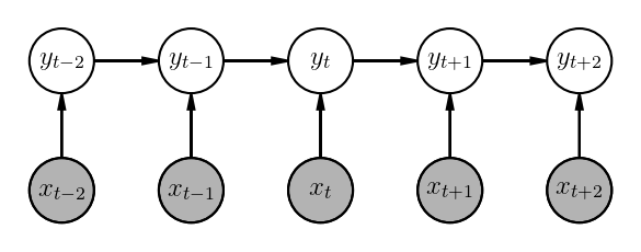
A trigram MEMM represents the conditional distribution the following way:
\[p(\underline{y_{1:T}}|\underline{x_{1:T}}) = \prod_{t=1}^{T}p(y_t|y_{t-1},y_{t-2}, \underline{x_{1:T}})\]and
\[score(y_{t-2},y_{t-1}, y_t, \underline{x_{1:T}}, t) = \sum_{k=1}^{K} w_k \cdot f_k(y_{t-2},y_{t-1}, y_t, \underline{x_{1:T}}, t) \\ p(y_t|y_{t-1},y_{t-2}, \underline{x_{1:T}}, \underline{\theta}) = \frac{e^{score(y_{t-2},y_{t-1}, y_t, \underline{x_{1:T}}, t)}}{\sum_{\widetilde{y}} e^{score(y_{t-2},y_{t-1}, \widetilde{y}, \underline{x_{1:T}}, t)}}\]where $\underline{\theta} = \underline{w_{1:K}}$ are the parameters of the model.
You may have noticed, we are incorporating richer context in the scoring functions - apart from preceeding two tags, we are also considering the whole input token sequence as well as the position information. Thus, while predicting a tag for a given position $t$, you can also look at the future tokens. For e.g. if the next token is a noun, then the likelihood of current tag being an adjective or determiner goes up. This representation is not possible in HMMs due the the way they are factorized.
The parameter learning and optimization procedure for MEMMs looks very similar to that for HMMs. Same goes with decoding, which has a nice recursive structure, thus allowing us to use Dynamic Programming.
Label Bias Problem in MEMMs
I possibly cannot do any better job of explaining the label bias problem in MEMMs than has been done by Awni Hannun in this excellent write-up. Essentially, the crux of the problem with MEMMs is that:
- There is no way to recover from past mistakes as the decoding process moves ahead in the time dimension. Which state is transitioned to every time step is decided “locally”.
- Often times, observations may have little effect in which states are transitioned to as states with fewer out-degrees are preferred as they don’t reduce the overall probability too much.
Conditional Random Fields (CRF)
We will talk about linear chain CRFs in this section. The equations for CRFs look like the following:
\[p(\underline{y_{1:T}}|\underline{x_{1:T}}) = \frac{e^{score(\underline{y_{1:T}}, \underline{x_{1:T}})}}{\sum_{\underline{\widetilde{y}_{1:T}}}e^{score(\underline{\widetilde{y}_{1:T}}, \underline{x_{1:T}})}}\]where
\[score(\underline{y_{1:T}}, \underline{x_{1:T}}) = \sum_{t=1}^{T+1}score(y_{t-1}, y_t, x_t, t)\]The main difference here from MEMMs is that the probability is not being normalized locally at every state, but rather globally. This allows us to rectify some of the issues with label bias and not being able to correct previous mistakes as selection is being done in a holistic way. The downside is that the normalization needs to be carried out over all possible tag sequences, which can be exponentially difficult. The decoding algorithm for CRFs is also more expensive compared to HMMs and MEMMs.
The score component is typically broken down into two components for a linear chain CRF:
\[score(y_{t-1}, y_t, x_t, t) = score_{TRANS}(y_t, y_{t-1}) + score_{EMIT}(y_t, x_t, t)\]$score_{TRANS}(y_t, y_{t-1})$ can be stored in a transition score matrix.
\[score_{TRANS}(y_t, y_{t-1}) = T[y_{t-1}, y_t]\]$score_{EMIT}(y_t, x_t, t)$ can be computed by a recurrent Nueral Networks such as an RNN or LSTM by casting it’s hidden state into a vectors of scores for every state $y_t$.
\[h_t, c_t = \text{LSTM}(x_t, (h_{t-1}, c_{t-1})) \\ y_{scores} = \textbf{W}\cdot h_t + b \\ score_{EMIT}(y_t, x_t, t) = y_{scores}[y_t]\]The factor graph for a linear chain CRF looks like the following:
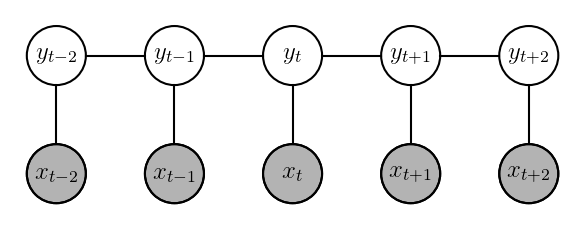
A natural question is, why use CRFs on top of an LSTM? Why not just use LSTM’s output ($y_{scores}$) to predict a tag at each timestep? While that would certainly work and yield reasonable accuracy, CRFs often impose tigher restrictions on the output, thus improving accuracy further. For e.g., in case of BIO tagging for NER prediction, CRFs can learn the contraints that a one or more I tags always follows a B tag without any O gaps in between.
Here is a PyTorch tutorial about using CRFs with BiLSTMs. Warning - it’s pretty involved!